Noisy Circuit Simulation

Overview

In this notebook, we will show how to perform noisy circuit simulation using TenCirChem. The hydrogen molecule \(\rm{H}_2\) is used for the demonstration. Using parity transformation, the system corresponds to 2 qubits. We will firstly illustrate the workflow step by step, and then use well-wrapped high-level interfaces to complete the same task with much fewer lines of code. We will also show it is possible to use Qiskit ansatz directly in TenCirChem. In the end, we study the effect of gate noise and the number of measurement shots on the accuracy and uncertainty of VQE.

Setup

TenCirChem uses the HEA class for noisy circuit simulation, which has a different set of interfaces from the UCC classes. A primary reason is that all ideal UCC circuits are too large for both noisy circuit simulation and execution on state of the art quantum devices. Consequently, usually hardware-efficient ansatz (HEA) have to be adopted for such tasks. Another reason is that inherently the workflow for the noiseless UCC circuit simulation and noisy HEA circuit simulation are very different.

from tencirchem import HEA
from tencirchem.molecule import h2

Define the Hamiltonian

The first difference between UCC and HEA is that the HEA class is not initialized by molecular inputs. Rather, HEA accepts the Hamiltonian in openfermion.QubitOperator form and the circuit ansatz for inputs. To facilitate defining the Hamiltonian, the UCC class provides several useful shortcuts via class attributes.

from tencirchem import UCCSD

uccsd = UCCSD(h2)
# Hamiltonian as openfermion.FermionOperator
h_fermion_op = uccsd.h_fermion_op
h_fermion_op

0.7141392859919029 [] +
-1.2527052599711868 [0^ 0] +
-0.48227117798977825 [0^ 1^ 0 1] +
-0.6745650967143663 [0^ 2^ 0 2] +
-0.18126641677772592 [0^ 2^ 1 3] +
-0.6635375947675042 [0^ 3^ 0 3] +
-0.18126641677772592 [0^ 3^ 1 2] +
-0.47569770336145906 [1^ 1] +
-0.18126641677772592 [1^ 2^ 0 3] +
-0.6635375947675038 [1^ 2^ 1 2] +
-0.18126641677772592 [1^ 3^ 0 2] +
-0.6974673850129379 [1^ 3^ 1 3] +
-1.2527052599711868 [2^ 2] +
-0.48227117798977825 [2^ 3^ 2 3] +
-0.47569770336145906 [3^ 3]

from tencirchem import parity

# use parity transformation for qubit Hamiltonian and remove 2 qubits
h_qubit_op = parity(h_fermion_op, uccsd.n_qubits, uccsd.n_elec)
h_qubit_op

-0.33948675952516477 [] +
0.18126641677772592 [X0 X1] +
-0.39422935037950685 [Z0] +
-0.01123932304807404 [Z0 Z1] +
0.3942293503795067 [Z1]

An alternative approach is to use openfermion tools such as openfermion.MolecularData.

Define the ansatz

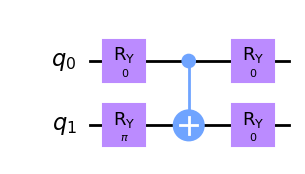
Next, define the ansatz using TensorCircuit. A 1-layer \(R_y\) ansatz composed of 4 parameters is constructed. A TensorCircuit ansatz is a function that has one argument (the circuit parameters) and returns the parameterized circuit.

import numpy as np
from tensorcircuit import Circuit

# the ansatz
n_qubits = 2
init_guess = [0, np.pi, 0, 0]


def get_circuit(params):
    c = Circuit(n_qubits)
    # the ansatz body
    c.ry(0, theta=params[0])
    c.ry(1, theta=params[1])
    c.cnot(0, 1)
    c.ry(0, theta=params[2])
    c.ry(1, theta=params[3])
    return c


get_circuit(init_guess).draw(output="mpl")

Noisy simulation with the HEA class

The rest of the workflow is similar to UCC: create an HEA instance, run the kernel and print the summary.

By using the "tensornetwork-noise" engine, a depolarizing noise with probability \(p=0.02\) for the CNOT gate is added

\[\mathcal{E}(\rho) = (1 - p)\rho + \frac{p}{15} \sum_{i} P_j \rho P_j\]

Here \(P_j\) are two qubit Pauli matrices except \(I\). An alternative form is

\[\mathcal{E}(\rho) = \frac{16p}{15} \frac{I}{4} + (1 - \frac{16p}{15}) \rho\]

When \(p=0\), no error is introduced. When \(p=\frac{15}{16}\), this is a completely depolarizing channel. If \(\rho\) is a pure state, the gate fidelity is \(1-\frac{4}{5}p\), which is is approximately 98% if \(p=0.02\).

The gradient of the parameters is evaluated by the parameter-shift rule and not by auto-differentiation.

hea = HEA(h_qubit_op, get_circuit, init_guess, engine="tensornetwork-noise")
hea.kernel()
hea.print_summary()

############################### Circuit ###############################
   #qubits  #gates  #CNOT  #multicontrol  depth #FLOP
0        2       5      1              0      3    96
######################### Optimization Result #########################
            e: -1.1202549357480136
          fun: array(-1.12025494)
     hess_inv: <4x4 LbfgsInvHessProduct with dtype=float64>
   init_guess: array([0.        , 3.14159265, 0.        , 0.        ])
          jac: array([5.16941739e-10, 5.55111512e-17, 0.00000000e+00, 0.00000000e+00])
      message: 'CONVERGENCE: NORM_OF_PROJECTED_GRADIENT_<=_PGTOL'
         nfev: 5
          nit: 3
         njev: 5
     opt_time: 0.25640320777893066
 staging_time: 1.1920928955078125e-06
       status: 0
      success: True
            x: array([-2.25973122e-01,  3.14159265e+00, -6.82347069e-17,  7.19412730e-17])

Different noise models can be specified using the NoiseConf class from TensorCircuit. Here we show a customized noise model with \(p=0.25\) and gate fidelity of 80%. The energy obtained is higher than the \(p=0.02\) result.

from tensorcircuit.noisemodel import NoiseConf
from tensorcircuit.channels import isotropicdepolarizingchannel

engine_conf = NoiseConf()
# larger noise, corresponding to 80% fidelity
channel = isotropicdepolarizingchannel(p=0.25, num_qubits=2)
engine_conf.add_noise("cnot", channel)

hea = HEA(h_qubit_op, get_circuit, init_guess, engine="tensornetwork-noise", engine_conf=engine_conf)
hea.kernel()
hea.print_summary()

############################### Circuit ###############################
   #qubits  #gates  #CNOT  #multicontrol  depth #FLOP
0        2       5      1              0      3    96
######################### Optimization Result #########################
            e: -0.9245310332616318
          fun: array(-0.92453103)
     hess_inv: <4x4 LbfgsInvHessProduct with dtype=float64>
   init_guess: array([0.        , 3.14159265, 0.        , 0.        ])
          jac: array([ 3.87354315e-10, -5.55111512e-17, -5.55111512e-17,  0.00000000e+00])
      message: 'CONVERGENCE: NORM_OF_PROJECTED_GRADIENT_<=_PGTOL'
         nfev: 5
          nit: 3
         njev: 5
     opt_time: 0.25928783416748047
 staging_time: 9.5367431640625e-07
       status: 0
      success: True
            x: array([-2.25973122e-01,  3.14159265e+00, -1.83807579e-16, -9.76918418e-17])

The "tensornetwork-noise" engine does not consider measurement uncertainty. In other words, the engine assumes that infinite shots are taken for each term in the Hamiltonian. In order to take measurement uncertainty into account, use the "tensornetwork-noise&shot" engine. By default the number of shots for each term is 4096. Note that the engine is significantly slower to run due to the computational overhead. Similar to the UCC class, the HEA class supports switching engine at runtime. The following example shows that by increasing measurement shots the energy uncertainty is suppressed.

# default shots is 4096
print("shots number: 4096")
for i in range(5):
    print(hea.energy(engine="tensornetwork-noise&shot"))
print("shots number: 4096 * 128")
hea.shots = 4096 * 128
for i in range(5):
    print(hea.energy(engine="tensornetwork-noise&shot"))

shots number: 4096
-0.9187451689899536
-0.9285959899718158
-0.9285225235212169
-0.9349106044977904
-0.9264353453475235
shots number: 4096 * 128
-0.9250756148331946
-0.9245772630966033
-0.9238598336661094
-0.924377692124025
-0.923522568588401

Finally, noiseless results are available by using the "tensornetwork" engine, in which case the energy is in exact agreement with the FCI energy for the hydrogen molecule system.

hea.energy(engine="tensornetwork"), uccsd.e_fci

(-1.1372744055294381, -1.1372744055294384)

Built-in ansatz, UCC ansatz and Qiskit ansatz

TenCirChem has implemented the \(R_y\) ansatz. We can rebuild the HEA instance using the HEA.ry function, which builds the qubit Hamiltonian and the \(R_y\) ansatz automatically, and then run the kernel. Note that the default initial guess is randomly generated. The result is exactly the same as what we’ve done step by step in the above code.

hea = HEA.ry(uccsd.int1e, uccsd.int2e, uccsd.n_elec, uccsd.e_core, n_layers=1, engine="tensornetwork-noise")
hea.init_guess = init_guess
hea.kernel()

-1.1202549357480136

If desired, the UCC ansatz defined in the UCC class can be fed into the HEA class for noisy circuit simulation. Note that TenCirChem by default uses a multi-qubit controlled \(R_y\) gate for UCC circuit simulation, which has to be decomposed into elementary gates first for actual execution on quantum computers. The gradient is turned off because parameter-shift rule is not applicable to the circuit. The energy obtained is significantly higher than HEA ansatz, because there are so many CNOT gates in the circuit.

from functools import partial

get_circuit = partial(uccsd.get_circuit, decompose_multicontrol=True)
hea = HEA(uccsd.h_qubit_op, get_circuit, uccsd.init_guess, engine="tensornetwork-noise")
hea.grad = "free"
hea.kernel(), get_circuit().gate_count(["cnot"])

(-0.8208126798813514, 18)

HEA also directly accepts qiskit parameterized circuit as input. While qiskit offers a rich library of circuits, TenCirChem offers much faster simulation speed and friendly user interfaces.

from qiskit import QuantumCircuit
from qiskit.circuit.library import TwoLocal

ansatz = QuantumCircuit(2)
ansatz = ansatz.compose(TwoLocal(2, rotation_blocks="ry", entanglement_blocks="cx", reps=1).decompose())
ansatz.draw(output="mpl")

hea = HEA(h_qubit_op, ansatz, init_guess, engine="tensornetwork-noise")
hea.kernel()

-1.1202549357480136

Effect of gate noise on VQE energy

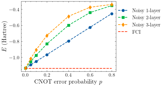
Here we show how the CNOT depolarizing error affects the optimized VQE energy. If a one-layer ansatz is adopted, the energy increases linearly with the error probability up to \(p=0.8\). This is a consequence of the special form of the ansatz: there’s only one CNOT gate in the circuit. Increasing the number of layers does not lead to more accurate energy estimation. Rather, the noise caused by more CNOT gates deteriorates the result.

from tencirchem import get_noise_conf, set_backend

# cnot error probabilities
error_probs = [0.001, 0.05, 0.10, 0.20, 0.40, 0.60, 0.80]
# number of layers in the ansatz
n_layers = [1, 2, 3]
e_list = []
# record run time
import time

time1 = time.time()
for n_layer in n_layers:
    hea = HEA.ry(uccsd.int1e, uccsd.int2e, uccsd.n_elec, uccsd.e_core, n_layers=n_layer, engine="tensornetwork-noise")
    # set HF init state
    hea.init_guess = np.zeros_like(hea.init_guess)
    hea.init_guess[1] = np.pi
    for error_prob in error_probs:
        hea.engine_conf = get_noise_conf(error_prob)
        e = hea.kernel()
        e_list.append(e)
e_array = np.array(e_list).reshape(3, -1)
time.time() - time1

14.445068836212158

from matplotlib import pyplot as plt
import mpl_config


plt.plot(error_probs, e_array[0], marker="o", linestyle="--", label="Noisy 1-layer")
plt.plot(error_probs, e_array[1], marker="s", linestyle="--", label="Noisy 2-layer")
plt.plot(error_probs, e_array[2], marker="d", linestyle="--", label="Noisy 3-layer")
plt.plot(error_probs, [uccsd.e_fci] * len(error_probs), linestyle="--", label="FCI")

plt.xlabel("CNOT error probability $p$")
plt.ylabel("$E$ (Hartree)")
plt.legend(loc=(1, 0.5))
plt.savefig("error-probability.pdf")

Effect of measurement shots on VQE energy uncertainty

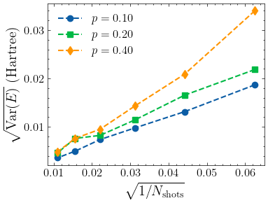
Here we show how measurement shots affect the standard deviation of the optimized VQE energy. As expected, the standard deviation is in linear relation with \(\sqrt{\frac{1}{N}}\). In general, increasing \(p\) causes a larger standard deviation of the energy, yet the effect is far less significant than adjusting \(N\).

hea = HEA.ry(uccsd.int1e, uccsd.int2e, uccsd.n_elec, uccsd.e_core, n_layers=1, engine="tensornetwork-noise")
hea.kernel()
# cnot error probabilities
error_probs = [0.10, 0.20, 0.40]
# number of measurement shots
shots_list = [2**i for i in range(8, 14)]
e_list = []
# record run time
time1 = time.time()
for error_prob in error_probs:
    for shots in shots_list:
        hea.engine_conf = get_noise_conf(error_prob)
        hea.shots = shots
        e = []
        for i in range(64):
            e.append(hea.energy(engine="tensornetwork-noise&shot"))
        e_list.append(e)
e_array = np.array(e_list).reshape(len(error_probs), -1, 64)
time.time() - time1

11.673604011535645

plt.plot(np.array(shots_list) ** (-0.5), e_array.std(axis=2)[0], marker="o", label="$p=0.10$", linestyle="--")
plt.plot(np.array(shots_list) ** (-0.5), e_array.std(axis=2)[1], marker="s", label="$p=0.20$", linestyle="--")
plt.plot(np.array(shots_list) ** (-0.5), e_array.std(axis=2)[2], marker="d", label="$p=0.40$", linestyle="--")
plt.xlabel(r"$\sqrt{1 / N_{\rm{shots}}}$")
plt.ylabel(r"$\sqrt{\textrm{Var}(E)}$ (Hartree)")
plt.legend()
plt.savefig("uncertainty.pdf")